Mapping to a 't'(map) (Last updated: 2025-06-13)
the tmap package for beautiful static and interactive maps with R
More maps of the Highlands?
Yep, same as last time, but no need to install dev versions of anything, we can get awesome maps courtesy of the tmap package.
Get the shapefile from the last post
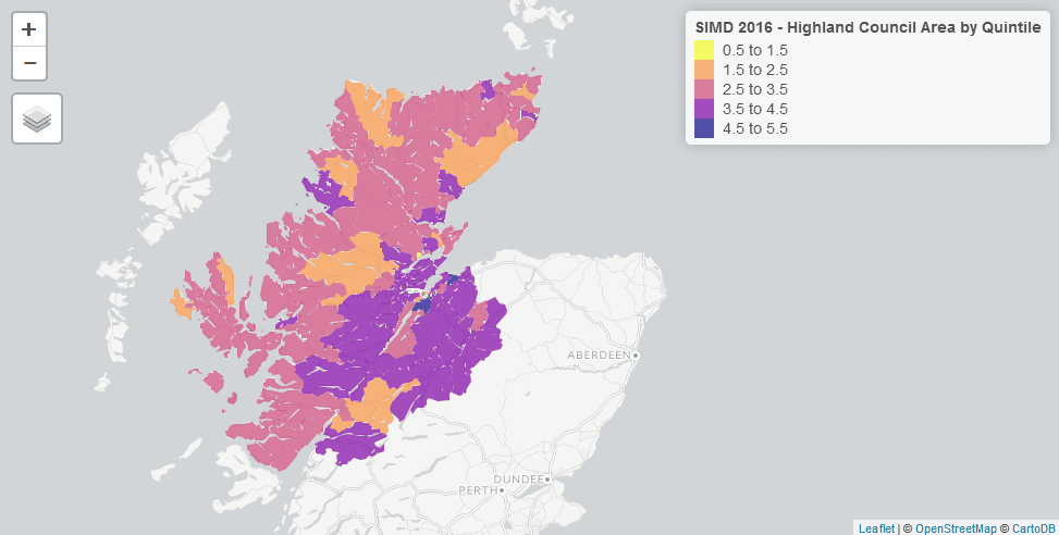
library(tmap) library(tmaptools) library(viridis) scot <- read_shape("SG_SIMD_2016.shp", as.sf = TRUE) highland <- (scot[scot$LAName=="Highland", ]) #replicate plot from previous blog post: quint <- tm_shape(highland) + tm_fill(col = "Quintile", palette = viridis(n = 5, direction = -1, option = "C"), fill.title = "Quintile", title = "SIMD 2016 - Highland Council Area by Quintile") quint # plot ttm() #switch between static and interactive - this will use interactive quint # or use last_map() # in R Studio you will find leaflet map in your Viewer tab ttm() # return to plotting The results:
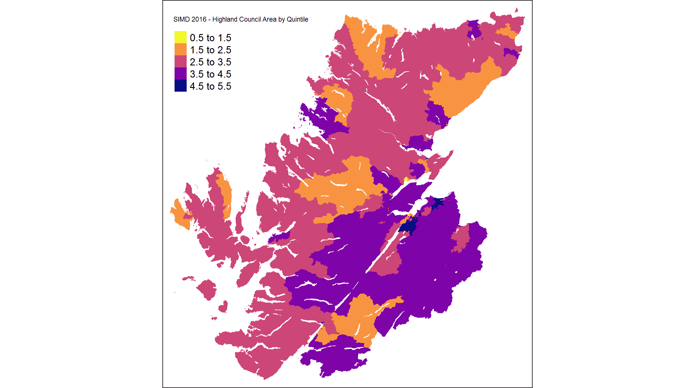
One really nice thing is that because the polygons don’t have outlines, the DataZones that are really densely packed still render nicely - so no ‘missing’ areas.
A static image of the leaflet map:
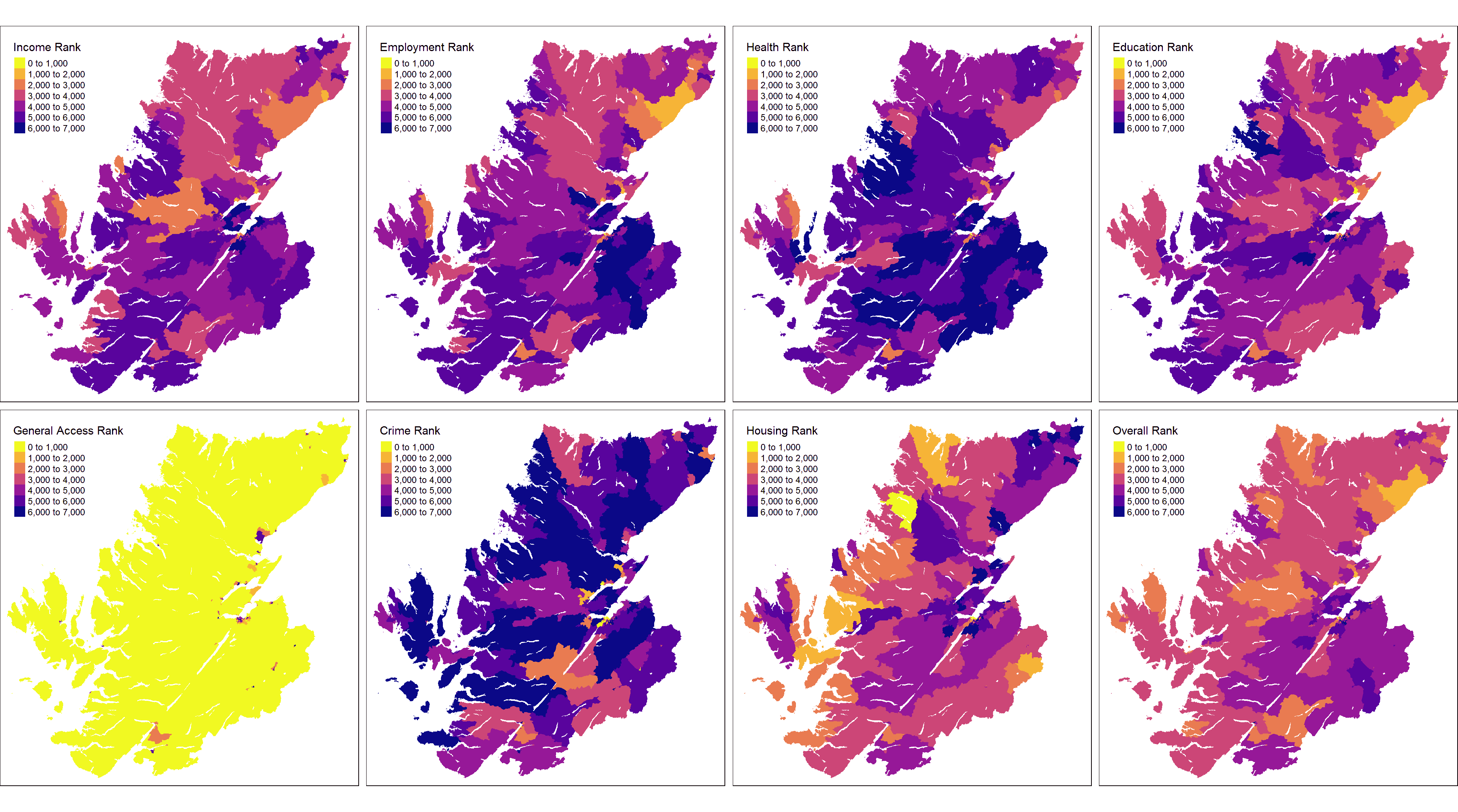
Here I take the main domain ranks (each of which summarises a number of other metrics) for all the Highland data zones, and the overall SIMD rank, and create a small multiple. The Highland region ranks very lowly compared to the rest of Scotland for access to services (e.g.average drive times to school, GP etc, and average public transport times to the same). No surprise.
However, it looks pretty good for Health and Employment in most areas (remember the ranks are assigned to all datazones in Scotland):
small_mult<- tm_shape(highland) + tm_fill(col = c("IncRank","EmpRank","HlthRank","EduRank", "GAccRank","CrimeRank","HouseRank","Rank"), palette = viridis(n = 5, direction = -1, option = "C"), title=c("Income Rank", "Employment Rank","Health Rank","Education Rank", "General Access Rank","Crime Rank", "Housing Rank","Overall Rank")) small_mult
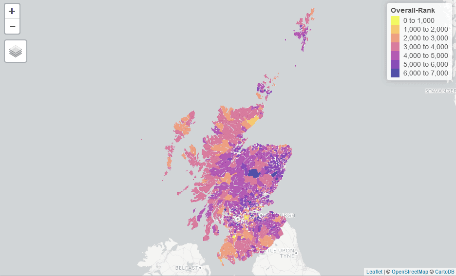
Let’s take a look at Scotland as a whole, as I assume everyone’s pretty bored of the Highlands by now:
#try a map of scotland scotplot <- tm_shape(scot) + tm_fill(col = "Rank", palette = viridis(n = 5, direction = -1, option = "C"), fill.title = "Overall Rank", title = "Overall-Rank") scotplot # bit of a monster 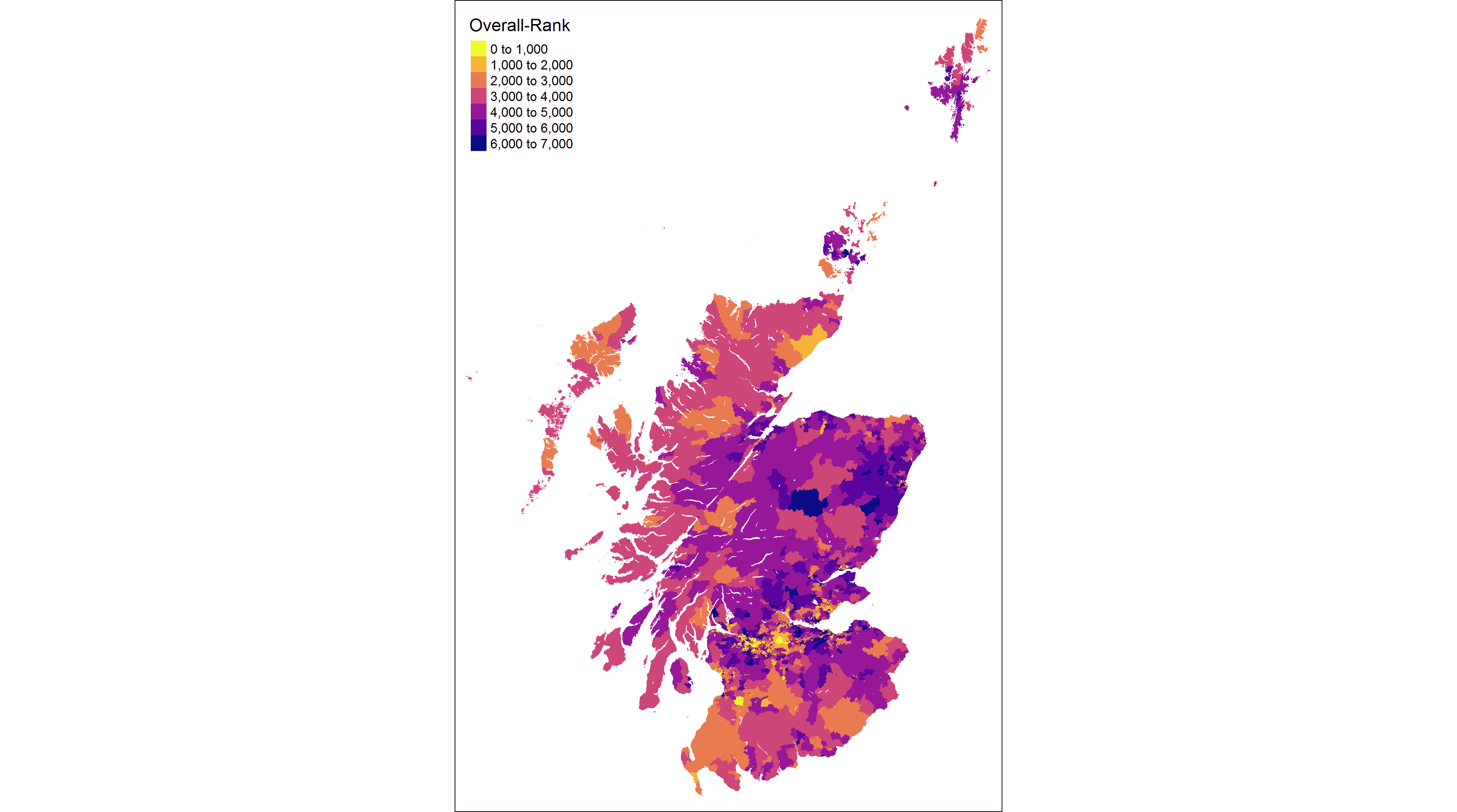
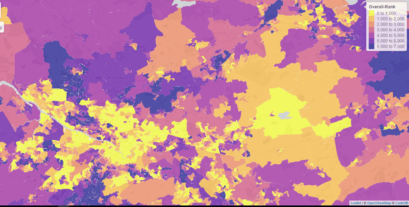
With the interactive plot, we can really appreciate the density of these datazones in the Central belt.
Here, I’ve zoomed in a bit on the region around Glasgow, and then zoomed in some more:

I couldn’t figure out how to host the leaflet map within the page (Jekyll / Github / Leaflet experts please feel free to educate me on that :) ) but, given the size of the file, I very much doubt I could have uploaded it to Github anyway.
Thanks to Roger Bivand (@RogerBivand) for getting in touch and pointing me towards the tmap package! It’s really good fun and an easy way to get interactive maps up and running. There are many more refinements that can be made to the plots, but you can look into those yourself ;).
Code and plots can be found here : SIMD tmap